library(readr) # read and write tabular data
library(dplyr) # manipulate data
library(lubridate) # manipulate dates
library(ggplot2) # create data visualizations
library(sf) # handle vector geospatial data
library(mapview) # create interactive maps
library(basemaps) # add basemap
library(here) # file paths

source(here('scripts/data_utils.R'))Additional Analysis
In this section, we will show a few more examples of maps, charts, and code.
For more examples of charts and graphs visit R Graph Gallery.
source(here('scripts/data_utils.R')) loads a script file with custom functions created for this workshop.
There is a bug with sf https://github.com/r-spatial/sf/issues/1762. This bit of code is fix for the bug.
sf_use_s2(FALSE)Spherical geometry (s2) switched offFirst, we need to read data from the CNC iNaturalist observation file.
inat_data <- read_csv(here('data/cleaned/cnc-los-angeles-observations.csv.zip'))Let’s add a year column to iNaturalist data.
inat_year <- inat_data |>
  mutate(year = year(observed_on))
Let’s add a geometry column
inat_sf <- inat_data |>
  st_as_sf(coords = c("longitude", "latitude"),   crs = 4326) |>
  select(user_login, common_name, scientific_name, observed_on,  url, quality_grade)
Dodged bar charts
To create side-by-side dodged bar charts, use position=position_dodge()
ggplot(data = inat_year ,
       mapping = aes(x = year, fill = quality_grade))  +
geom_bar(position = position_dodge(preserve = 'single')) 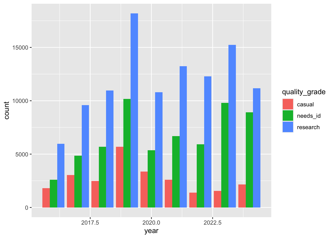
Multiple line charts
If we want a chart with multiple lines, we need to create a data frame with three columns: one column x axis, one column for y axis, and one column for color.
year_quality_count <- inat_data |>
  mutate(year = year(observed_on))  |>
  count(year, quality_grade,  name='count')

year_quality_count
# A tibble: 27 × 3
year quality_grade count
<dbl> <chr> <int>
1 2016 casual 1819
2 2016 needs_id 2605
3 2016 research 5968
4 2017 casual 3045
5 2017 needs_id 4855
6 2017 research 9595
7 2018 casual 2492
8 2018 needs_id 5698
9 2018 research 10974
10 2019 casual 5696
# ℹ 17 more rowsggplot(data = year_quality_count,
mapping = aes(x = year, y = count, color = quality_grade)) +
geom_line()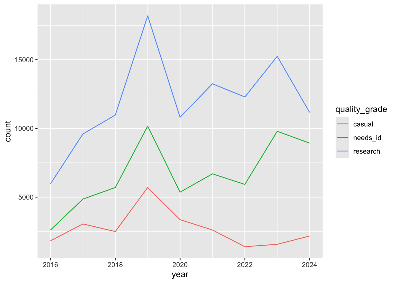
Multiple charts
Each geom_ adds a layer to the chart. We can have multiple chart layers in one chart by having multiple geom_.
Let’s create a bar and line chart that uses the same data and mapping.
inat_year_count <- inat_data |>
  mutate(year = year(observed_on)) |>
  count(year, name='count')

inat_year_count
# A tibble: 9 × 2
year count
<dbl> <int>
1 2016 10392
2 2017 17495
3 2018 19164
4 2019 34057
5 2020 19524
6 2021 22549
7 2022 19597
8 2023 26602
9 2024 22258ggplot(data = inat_year_count,
mapping = aes(x = year, y = count)) +
geom_col() +
geom_line()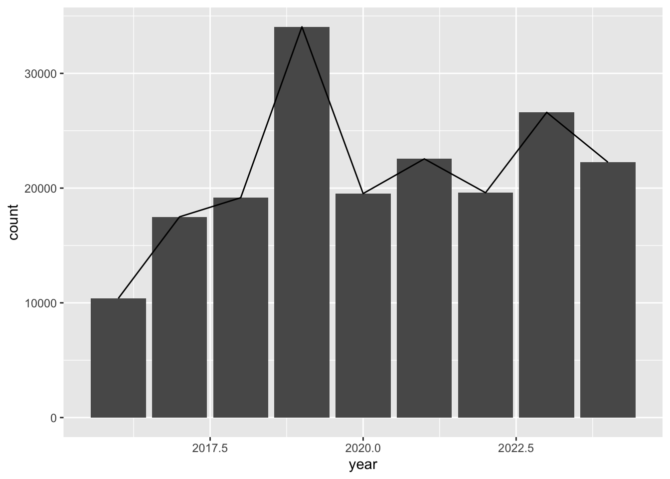
Let’s create a dodged bar and line chart that uses the different data and different mapping. Instead of putting the information inside ggplot(), we put information in each geom_.
ggplot() +
  geom_bar(data = inat_year ,
       mapping = aes(x = year, fill = quality_grade),
       position = position_dodge(preserve = 'single')) +
  geom_line(data = inat_year_count,
       mapping = aes(x = year, y = count))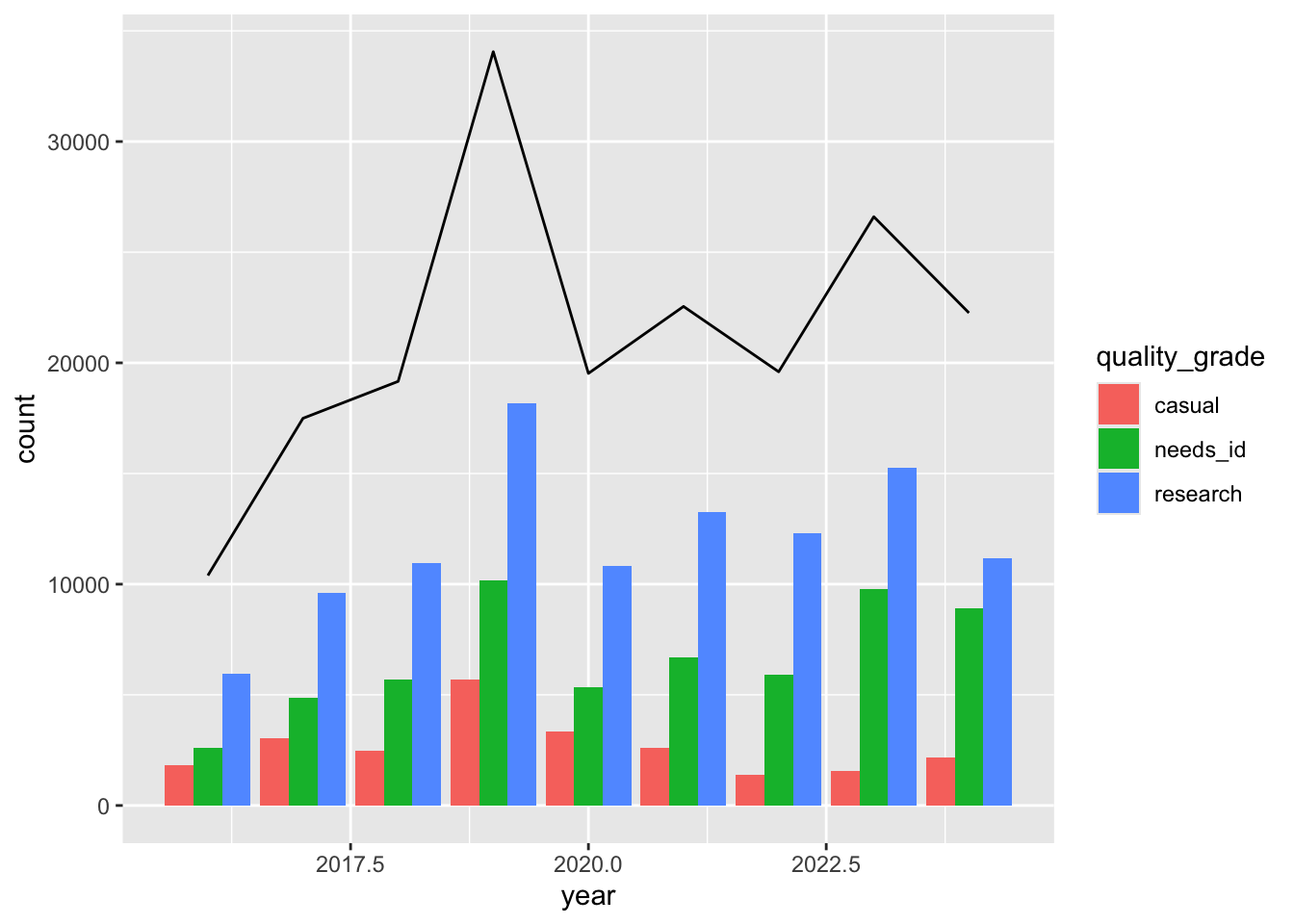
Adding labels and basemaps to ggplot map
Let’s get the observation counts for neighborhoods around Exposition Park
la_neighborhoods_sf <- read_sf(here('data/raw/la_times_la_county_neighborhoods.json'))Get Exposition Park neighborhood
expo_park_sf <- la_neighborhoods_sf |>
  filter(name=='Exposition Park')

expo_park_sf
Simple feature collection with 1 feature and 2 fields
Geometry type: MULTIPOLYGON
Dimension: XY
Bounding box: xmin: -118.3181 ymin: 34.01081 xmax: -118.2797 ymax: 34.02571
Geodetic CRS: WGS 84
# A tibble: 1 × 3
name slug geometry
* <chr> <chr> <MULTIPOLYGON [°]>
1 Exposition Park exposition-park (((-118.3054 34.02571, -118.3048 34.02561, -1…Get neighborhoods surrounding Exposition Park
expo_area_sf <- st_filter(la_neighborhoods_sf, expo_park_sf)although coordinates are longitude/latitude, st_intersects assumes that they
are planarexpo_area_sf <- expo_area_sf |>
select(name)
expo_area_sfSimple feature collection with 7 features and 1 field
Geometry type: MULTIPOLYGON
Dimension: XY
Bounding box: xmin: -118.3357 ymin: 33.99301 xmax: -118.2505 ymax: 34.03781
Geodetic CRS: WGS 84
# A tibble: 7 × 2
name geometry
<chr> <MULTIPOLYGON [°]>
1 Adams-Normandie (((-118.309 34.03741, -118.3057 34.03731, -118.3015 34…
2 Exposition Park (((-118.3054 34.02571, -118.3048 34.02561, -118.3041 3…
3 Historic South-Central (((-118.2564 34.00481, -118.2564 34.00381, -118.2587 3…
4 Jefferson Park (((-118.309 34.03641, -118.3091 34.03491, -118.309 34.…
5 Leimert Park (((-118.3181 34.01461, -118.318 34.01091, -118.317 34.…
6 University Park (((-118.2828 34.01842, -118.2864 34.01841, -118.2892 3…
7 Vermont Square (((-118.2827 34.01111, -118.282 34.01101, -118.2815 34…Use custom function add_inat_count_to_boundary_sf() to count the number of iNaturalist observations per neighborhood.
expo_area_count_sf <- add_inat_count_to_boundary_sf(inat_sf, expo_area_sf, 'name')although coordinates are longitude/latitude, st_intersects assumes that they
are planar
although coordinates are longitude/latitude, st_intersects assumes that they
are planarexpo_area_count_sfSimple feature collection with 7 features and 2 fields
Geometry type: MULTIPOLYGON
Dimension: XY
Bounding box: xmin: -118.3357 ymin: 33.99301 xmax: -118.2505 ymax: 34.03781
Geodetic CRS: WGS 84
# A tibble: 7 × 3
name geometry observations_count
<chr> <MULTIPOLYGON [°]> <int>
1 Adams-Normandie (((-118.309 34.03741, -118.3057 34.… 132
2 Exposition Park (((-118.3054 34.02571, -118.3048 34… 3160
3 Historic South-Central (((-118.2564 34.00481, -118.2564 34… 139
4 Jefferson Park (((-118.309 34.03641, -118.3091 34.… 382
5 Leimert Park (((-118.3181 34.01461, -118.318 34.… 81
6 University Park (((-118.2828 34.01842, -118.2864 34… 1466
7 Vermont Square (((-118.2827 34.01111, -118.282 34.… 95Create map with labels that show counts per neighborhood.
ggplot(expo_area_count_sf, aes(label=paste0(name,': ', observations_count))) +
  geom_sf() +
  geom_sf_label(fill = "white" )
Warning in st_point_on_surface.sfc(sf::st_zm(x)): st_point_on_surface may not
give correct results for longitude/latitude data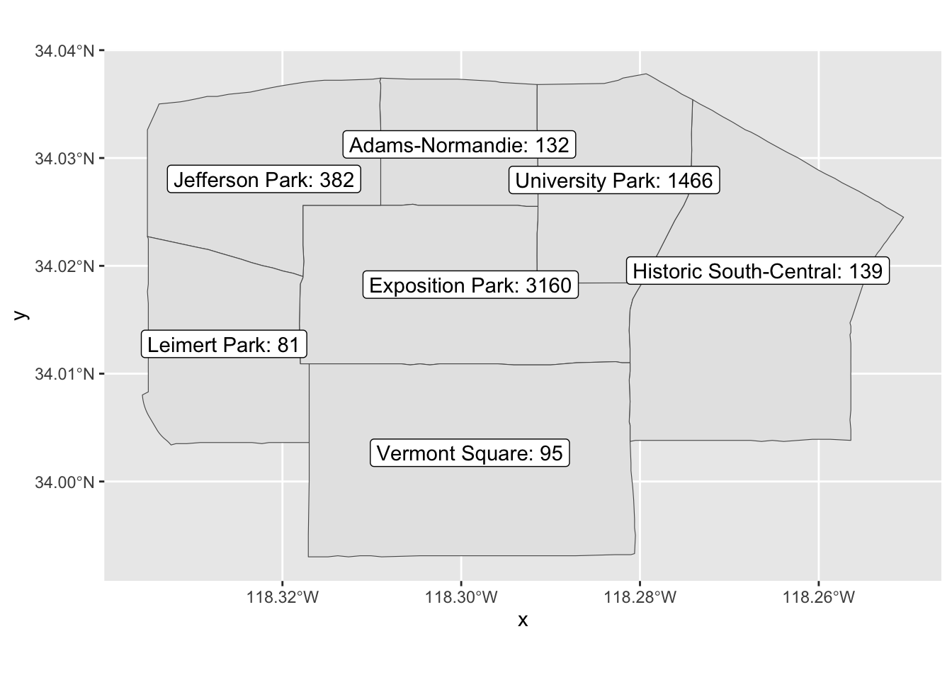
We can use basemaps package to add a basmap to ggplot maps.
Change crs to 3857 since basemaps package uses 3857.
expo_area_count_sf <- st_transform(expo_area_count_sf, crs = st_crs(3857))Create map with labels that show counts and basemap. Use basemap_gglayer() and scale_fill_identity() to add a basemap. Use aes(fill=alpha()) to make the fill for each neighborhood tranparent yellow.
ggplot(expo_area_count_sf) +
  basemap_gglayer(expo_area_count_sf) +
  scale_fill_identity() +
  geom_sf( mapping=aes(fill=alpha("yellow", .05))) +
  geom_sf_label( mapping=aes(label = paste0(name, ': ',observations_count)) )  +
  theme_void()
Loading basemap 'voyager' from map service 'carto'...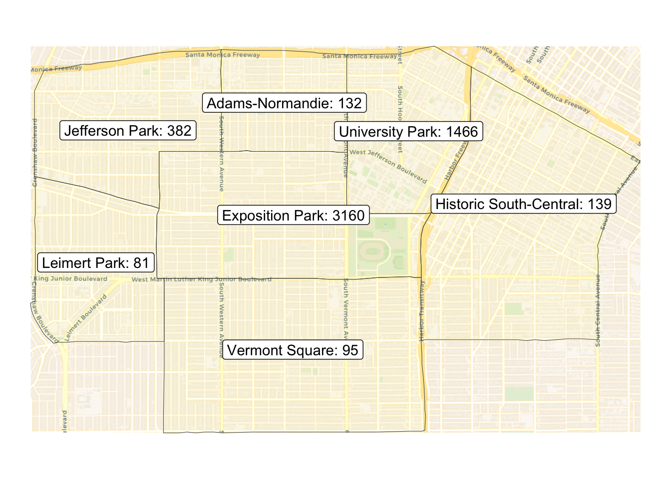
Compare iNaturalist observations per region to another value
We’ve provided a couple of maps with multiple boundaries that includes data values for each boundary. For instance the LA County Environmental Justice Screening Method has environmental impact scores for various areas in LA County.
Let’s compare iNaturalist observations with EJSM Cumulative Impact Score for each area.
ejsm_sf <- read_sf(here('data/raw/EJSM_Scores-shp/6cbc6914-690f-48ec-a54f-2649a8ddb321202041-1-139ir98.m1ys.shp'))

glimpse(ejsm_sf)
Rows: 2,343
Columns: 10
$ OBJECTID <int> 1, 2, 3, 4, 5, 6, 7, 8, 9, 10, 11, 12, 13, 14, 15, 16, 17, …
$ Tract_1 <dbl> 6037920336, 6037920044, 6037573003, 6037571704, 6037570403,…
$ CIscore <int> 10, 4, 13, 13, 17, 15, 14, 10, 11, 17, 15, 14, 12, 11, 13, …
$ HazScore <int> 3, 1, 5, 3, 5, 3, 4, 1, 3, 5, 4, 4, 4, 4, 5, 3, 2, 4, 5, 3,…
$ HealthScor <int> 1, 1, 3, 2, 3, 4, 2, 3, 4, 5, 4, 4, 4, 2, 2, 3, 3, 3, 5, 3,…
$ SVscore <int> 4, 1, 3, 4, 5, 4, 3, 4, 2, 3, 3, 4, 2, 3, 5, 3, 3, 3, 2, 2,…
$ CCVscore <int> 2, 1, 2, 4, 4, 4, 5, 2, 2, 4, 4, 2, 2, 2, 1, 5, 5, 5, 4, 3,…
$ Shape__Are <dbl> 2438559.8, 1470811.2, 652816.8, 699401.1, 831783.9, 617212.…
$ Shape__Len <dbl> 8124.373, 5545.298, 3310.744, 4113.477, 3887.000, 3495.394,…
$ geometry <MULTIPOLYGON [m]> MULTIPOLYGON (((-13194561 4..., MULTIPOLYGON (…Create a choropleth map using geom_sf() that shows Cumulative Impact Score.
ggplot(ejsm_sf, aes(fill = CIscore)) +
  geom_sf()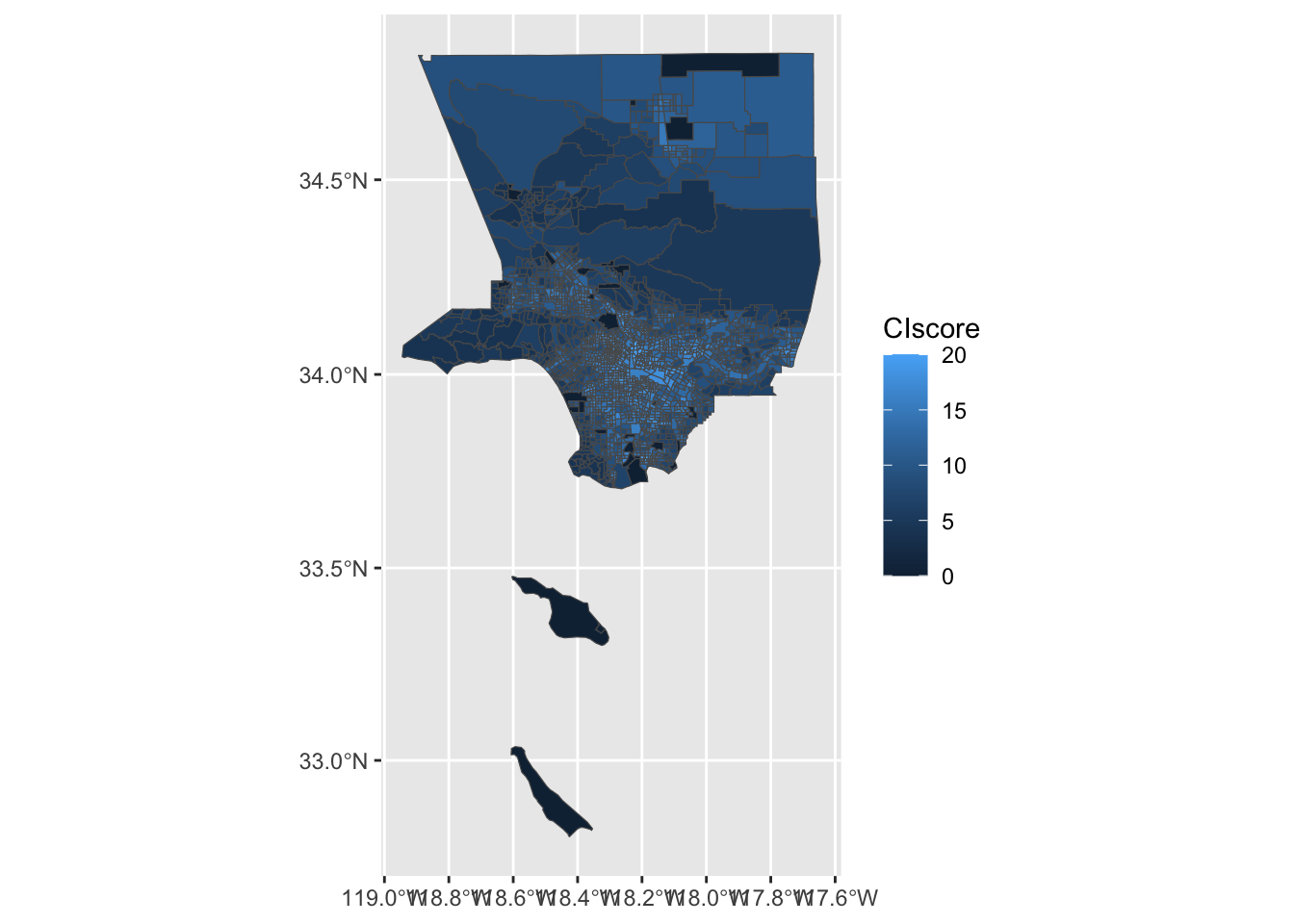
Check if the EJSM has the same CRS as the iNaturalist data.
st_crs(ejsm_sf) == st_crs(inat_sf)[1] FALSEUpdate CRS
ejsm_sf <- st_transform(ejsm_sf,  crs = st_crs(inat_sf))

st_crs(ejsm_sf) == st_crs(inat_sf)
[1] TRUEUse custom function add_inat_count_to_boundary_sf() to count the number of iNaturalist observations per region and add the count to ejsm_sf.
ejsm_inat_sf <- add_inat_count_to_boundary_sf(inat_sf, ejsm_sf, 'OBJECTID')although coordinates are longitude/latitude, st_intersects assumes that they
are planar
although coordinates are longitude/latitude, st_intersects assumes that they
are planarglimpse(ejsm_inat_sf)Rows: 2,343
Columns: 11
$ OBJECTID <int> 1, 2, 3, 4, 5, 6, 7, 8, 9, 10, 11, 12, 13, 14, 15, …
$ Tract_1 <dbl> 6037920336, 6037920044, 6037573003, 6037571704, 603…
$ CIscore <int> 10, 4, 13, 13, 17, 15, 14, 10, 11, 17, 15, 14, 12, …
$ HazScore <int> 3, 1, 5, 3, 5, 3, 4, 1, 3, 5, 4, 4, 4, 4, 5, 3, 2, …
$ HealthScor <int> 1, 1, 3, 2, 3, 4, 2, 3, 4, 5, 4, 4, 4, 2, 2, 3, 3, …
$ SVscore <int> 4, 1, 3, 4, 5, 4, 3, 4, 2, 3, 3, 4, 2, 3, 5, 3, 3, …
$ CCVscore <int> 2, 1, 2, 4, 4, 4, 5, 2, 2, 4, 4, 2, 2, 2, 1, 5, 5, …
$ Shape__Are <dbl> 2438559.8, 1470811.2, 652816.8, 699401.1, 831783.9,…
$ Shape__Len <dbl> 8124.373, 5545.298, 3310.744, 4113.477, 3887.000, 3…
$ geometry <MULTIPOLYGON [°]> MULTIPOLYGON (((-118.5288 3..., MULTIP…
$ observations_count <int> 11, NA, 4, 5, 3, 4, 4, 1, 11, 2, 5, 4, 16, 13, 21, …Another way to show iNaturalist counts per region is to draw a symbol in each area, and base the size of the symbol on the iNaturalist counts.
st_centroid from sf generates a point at the center of each region. Instead of drawing a polygon, we draw a point that represents the center of the polygon
centroid_sf <- st_centroid(ejsm_inat_sf) |>
  select(OBJECTID, observations_count)
Warning: st_centroid assumes attributes are constant over geometriesWarning in st_centroid.sfc(st_geometry(x), of_largest_polygon =
of_largest_polygon): st_centroid does not give correct centroids for
longitude/latitude dataglimpse(centroid_sf)Rows: 2,343
Columns: 3
$ OBJECTID <int> 1, 2, 3, 4, 5, 6, 7, 8, 9, 10, 11, 12, 13, 14, 15, …
$ observations_count <int> 11, NA, 4, 5, 3, 4, 4, 1, 11, 2, 5, 4, 16, 13, 21, …
$ geometry <POINT [°]> POINT (-118.5365 34.38503), POINT (-118.5163 …ggplot() +
geom_sf(data = centroid_sf) 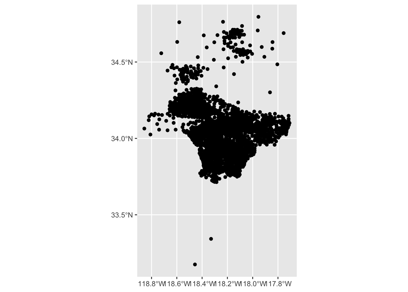
We can create a map that uses color to show CIscore per region, and uses circle size to show number iNaturalist observations per region.
We can use aes(size=<column>) to set the size of the circle based on observations_count column.
ggplot() +
  geom_sf(data=ejsm_inat_sf, aes(fill = CIscore)) +
  geom_sf(data = centroid_sf, aes(size = observations_count))
Warning: Removed 137 rows containing missing values or values outside the scale range
(`geom_sf()`).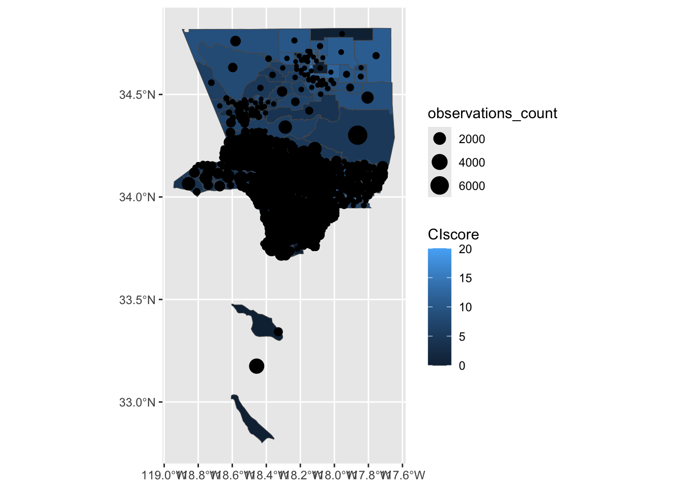
We can use cex to set the size of the circle based on observations_count column.
ejsm_inat_basic_sf <- ejsm_inat_sf |>
  select(CIscore)

mapview(ejsm_inat_basic_sf,
        zcol = 'CIscore') +
  mapview(centroid_sf, cex="observations_count",
          zcol="observations_count",legend=FALSE, col.regions='black')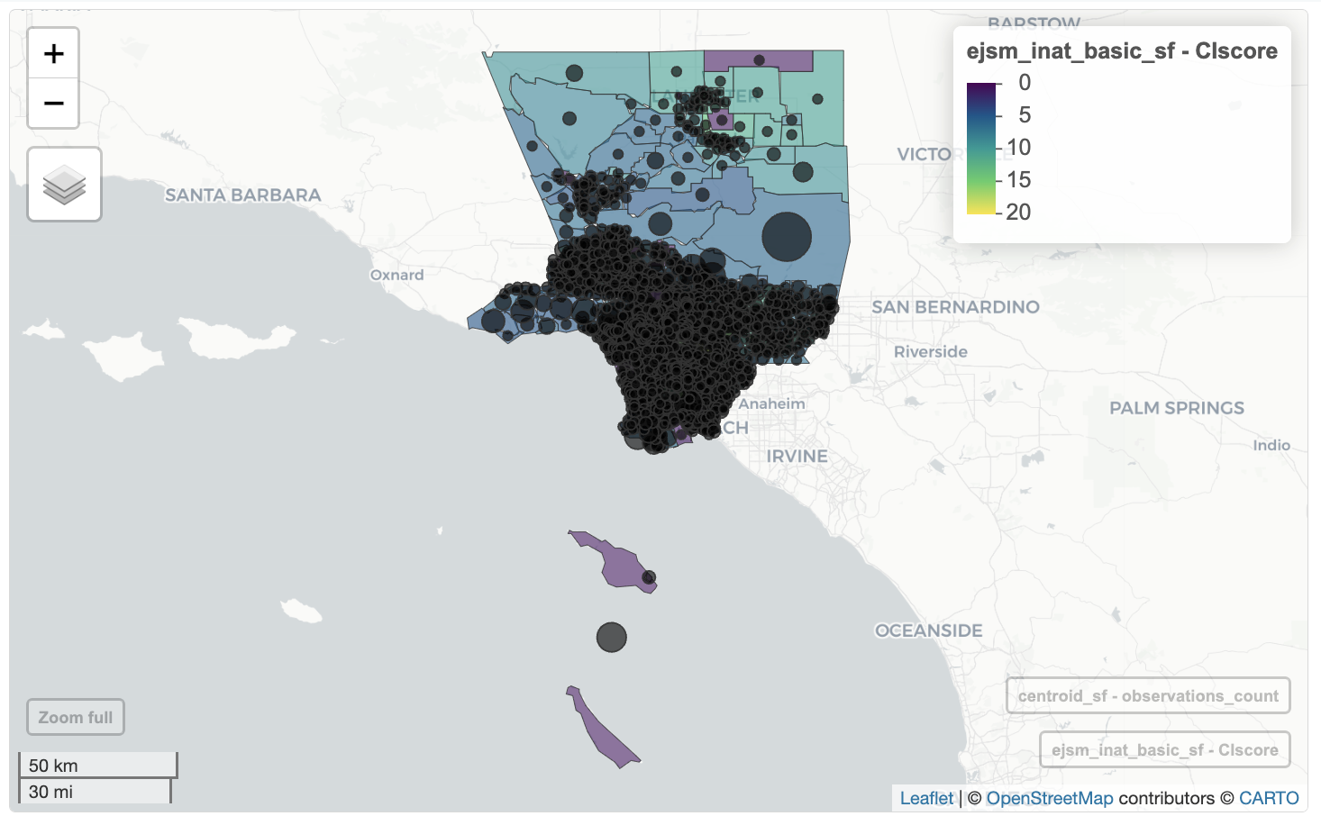
Download images
We provide a custom function to download images for a data frame of iNaturalist observations.
Just make sure you follow the license terms for the observations. Here’s a summary of the various Creative Commons licenses.
table(inat_data$license)
      CC-BY    CC-BY-NC CC-BY-NC-ND CC-BY-NC-SA    CC-BY-ND    CC-BY-SA
       5384      129677        1199        2934          35          79
        CC0
       4934
The observations are ordered from oldest date to newest date. Use filter() to select the observation you want. We can use slice to limit the number observation.
Use slice(start:end) to get observations from start row number to end row number. In this case we are getting the first five Western fence lizard observations with CCO license.
my_inat2 <- inat_data |>
  filter(common_name == 'Western Fence Lizard') |>
  filter(license == 'CC0') |>
  slice(1:5)

table(my_inat2$observed_on)
2016-04-15 2016-04-17 2016-04-18 2016-04-19 2017-04-17
         1          1          1          1          1
If you want to get a specified number of randomly selected rows, use slice_sample(n = <number>). In this case we are getting five random Western fence lizard observations with CCO license.
my_inat <- inat_data |>
  filter(common_name == 'Western Fence Lizard') |>
  filter(license == 'CC0') |>
  slice_sample(n=5)

table(my_inat$observed_on)
2016-04-17 2018-04-28 2021-05-01 2022-05-01 2022-05-02
         1          1          1          1          1
Once we have the observations we want, call custom function download_inaturalist_images() to download the images for the observations. The images are saved in the results directory. A new directory will be created for each scientific_name. The image name will contain the scientific name, observation id, username and license.
download_inaturalist_images(my_inat)