Intro to Data Analysis
Last updated on 2024-05-24 | Edit this page
Estimated time: 12 minutes
Overview
Questions
- How do we begin to analyze iNaturalist data?
Objectives
- Learn how to download data from iNaturalist
- Learn about the various ways to analyze data
iNaturalist data
When iNaturalist users add an observation through the iNaturalist app, that data is saved to the iNaturalist database. People can download the iNaturalist data as CSVs.
CSV is a text file format for tabular data. Each line represents one record. Each column represents a field. The fields are separated by commas.
The iNaturalist CSV has information about:
- the user who made observation
- the location of the observation
- the observed species
- links for photos, videos, sounds
Instructions to download iNaturalist data
Here’s a video that shows how to select and download data from iNaturalist.
To save time and ensure everyone at the workshop has the same data, here is a link to a CSV with iNaturalist City Nature Challenge Los Angeles data from 2013 to 2024.
More info about downloading iNaturalist observation data.
https://help.inaturalist.org/en/support/solutions/articles/151000169670
Analyzing data
It is difficult for people to see any patterns when reading rows after row of text. To make it easier to see patterns, we can use software to analyze tabular data.
Spreadsheet programs are computer application that people can use to view, edit, and analyze tabular data. The programs can do calculations and create charts. Examples include Excel and Google Sheets
Geographic information system (GIS) are computer application that people can use to view, edit and analyze geographic data. The programs can do calculations and create maps. Examples include ArcGIS and QGIS.
Programming languages allow people to write instructions to tell a computer to do stuff. We write these instructions in the form of code. We can write code to do calculations, create charts, and create maps. Example programming languages include R, Python, C.
This class uses R because it is a popular language in ecology research and other types of scientific research.
Example of analyzing iNaturalist data using R
Load software that will will need.
R
library(readr) # read and write tabular data
library(dplyr) # manipulate data
library(ggplot2) # create data visualizations
library(sf) # geospatial
library(lubridate) # manipulate dates
library(mapview) # create interactive maps
Load iNaturalist data from City Nature Challenge Los Angeles 2013-2023. There are over 170,000 observations.
R
inat <- read_csv("data/raw/observations-397280.csv")
OUTPUT
Rows: 171155 Columns: 39
── Column specification ────────────────────────────────────────────────────────
Delimiter: ","
chr  (23): observed_on_string, time_observed_at, time_zone, user_login, user...
dbl  (10): id, user_id, num_identification_agreements, num_identification_di...
lgl   (5): captive_cultivated, private_place_guess, private_latitude, privat...
date  (1): observed_on

ℹ Use `spec()` to retrieve the full column specification for this data.
ℹ Specify the column types or set `show_col_types = FALSE` to quiet this message.
Get the 10 most commonly observed ‘species’.
R
top_10 <- inat %>%
  filter(!is.na(scientific_name)) %>%
  select(common_name, scientific_name) %>%
  count(common_name, scientific_name, name='count')  %>%
  arrange(desc(count)) %>%
  slice(1:10)

top_10
OUTPUT
# A tibble: 10 × 3
common_name scientific_name count
<chr> <chr> <int>
1 Western Fence Lizard Sceloporus occidentalis 2970
2 dicots Magnoliopsida 1978
3 Western Honey Bee Apis mellifera 1818
4 plants Plantae 1665
5 Fox Squirrel Sciurus niger 1323
6 flowering plants Angiospermae 1151
7 House Finch Haemorhous mexicanus 1122
8 Mourning Dove Zenaida macroura 1078
9 Convergent Lady Beetle Hippodamia convergens 840
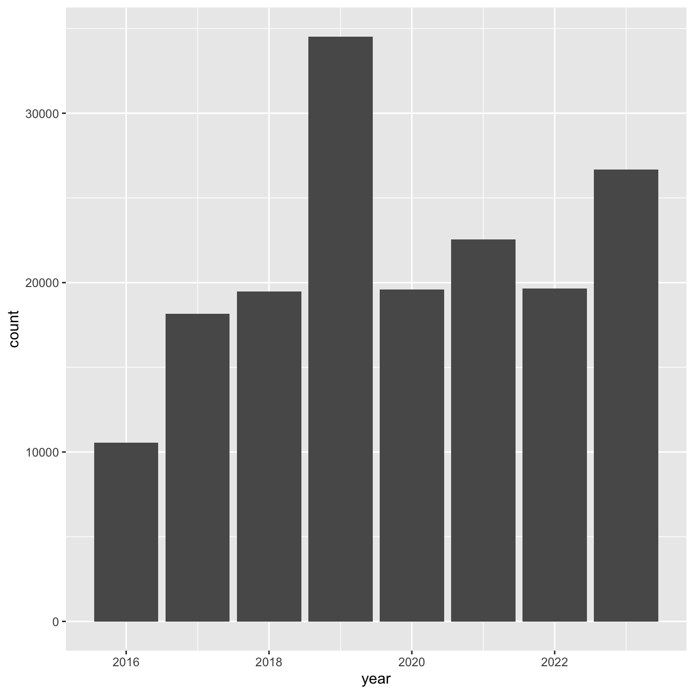
10 House Sparrow Passer domesticus 838Create a bar chart showing the number of observations per year.
R
inat %>%
  mutate(year = year(observed_on))  %>%
  group_by(year) %>%
  ggplot(aes(x = year)) +
  geom_bar()
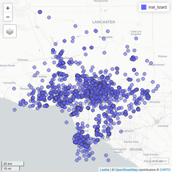
Create a map showing all the observations for Western Fence Lizard
https://www.ecologi.st/spatial-r/rdemo.html#converting-a-dataframe-into-a-spatial-object
R
inat_lizard <- inat %>%
  filter(!is.na(latitude) &
           !is.na(longitude) &
           !is.na(scientific_name)) %>%
  st_as_sf(coords = c("longitude", "latitude"),   crs = 4326, remove=FALSE) %>%
  select(id, user_login, common_name, scientific_name, observed_on,  url, longitude, latitude, geometry) %>%
  filter(common_name == 'Western Fence Lizard')


mapview(inat_lizard)