library(readr)
library(dplyr)

Attaching package: 'dplyr'

The following objects are masked from 'package:stats':

    filter, lag

The following objects are masked from 'package:base':

    intersect, setdiff, setequal, union

library(ggplot2)

I downloaded GBIF records for iNaturalist and Cornell Lab of Ornithology from 2015 to 2025 at Natural History Museum of Los Angeles County and Rose Garden.

QA raw GBIF data

nhm_raw_df <-read_tsv('../data/raw/0025996-250711103210423.csv')
dim(nhm_raw_df)

[1] 17755    50

rose_raw_df <-read_tsv('../data/raw/0025992-250711103210423.csv')
dim(rose_raw_df)

[1] 611  50

get count of taxon ranks

table(c(nhm_raw_df$taxonRank, rose_raw_df$taxonRank))

    FAMILY       FORM      GENUS    SPECIES SUBSPECIES    VARIETY 
        26          3        349      17873         89         26 

temp_nhm <- nhm_raw_df |> filter(institutionCode == 'CLO')
temp_rose <- rose_raw_df |> filter(institutionCode == 'CLO')

table(c(temp_nhm$taxonRank, temp_rose$taxonRank))

SPECIES 
  10651 

temp_nhm <- nhm_raw_df |> filter(institutionCode == 'iNaturalist')
temp_rose <- rose_raw_df |> filter(institutionCode == 'iNaturalist')

table(c(temp_nhm$taxonRank, temp_rose$taxonRank))

    FAMILY       FORM      GENUS    SPECIES SUBSPECIES    VARIETY 
        26          3        349       7222         89         26 

Get date for newest observation

 nhm_raw_df |> 
  filter(institutionCode == 'CLO') |> 
  select(eventDate) |> summary()

   eventDate                     
 Min.   :2014-01-06 00:00:00.00  
 1st Qu.:2016-07-12 00:00:00.00  
 Median :2018-12-26 00:00:00.00  
 Mean   :2018-12-13 19:37:31.60  
 3rd Qu.:2021-05-15 12:00:00.00  
 Max.   :2023-12-20 00:00:00.00  

 nhm_raw_df |> 
  filter(institutionCode == 'iNaturalist') |> 
  select(eventDate) |> summary()

   eventDate                     
 Min.   :2014-01-06 16:36:52.00  
 1st Qu.:2017-05-31 12:42:43.00  
 Median :2020-02-29 14:40:28.00  
 Mean   :2020-06-14 19:51:13.55  
 3rd Qu.:2023-06-22 11:39:06.00  
 Max.   :2025-06-17 14:16:54.00  

iNaturalist provides coordinateUncertaintyInMeters, CLO does not. Filter out iNaturalist records with high coordinateUncertaintyInMeters.

View distribution of coordinateUncertaintyInMeters.

temp_nhm <- nhm_raw_df |>
  filter(coordinateUncertaintyInMeters < 100)

ggplot(data = temp_nhm,  mapping = aes(x = coordinateUncertaintyInMeters)) +
  geom_histogram()

`stat_bin()` using `bins = 30`. Pick better value with `binwidth`.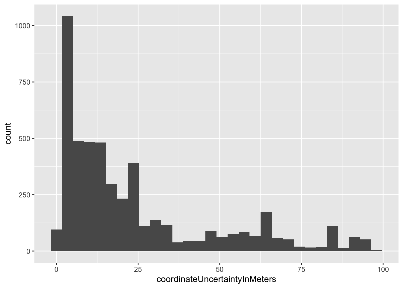

temp_rose <- rose_raw_df |>
  filter(coordinateUncertaintyInMeters < 100)

ggplot(data = temp_rose,  mapping = aes(x = coordinateUncertaintyInMeters)) +
  geom_histogram()

`stat_bin()` using `bins = 30`. Pick better value with `binwidth`.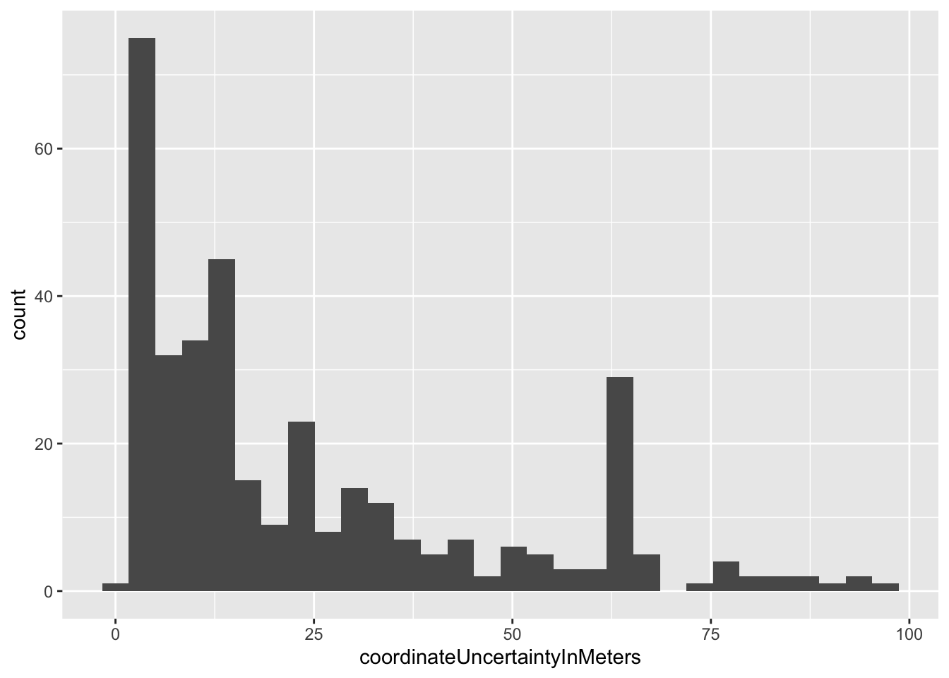

Count records by institutionCode.

table(nhm_raw_df$institutionCode)

        CLO iNaturalist 
      10594        7161 

table(rose_raw_df$institutionCode)

        CLO iNaturalist 
         57         554 

clean raw GBIF data

Here are the steps to clean the GBIF data.

• Select observations from 2104 to 2023 because GBIF does not currently have eBird records after December 2023.
• Select iNaturalist observations that have coordinate uncertainty of 100 meters or less. eBird observations do not provide coordinate uncertainty data.
• Select the iNaturalist observations where taxon rank is ‘FORM’, ‘SPECIES’, ‘SUBSPECIES’ or ‘VARIETY’. eBird only has ‘SPECIES’.

clean_gbif <- function(df) {
  df |>
  filter((institutionCode == 'iNaturalist' & 
            coordinateUncertaintyInMeters < 100 ) | 
           (institutionCode == 'CLO'))  |>
  filter(year %in% c(2014:2023)) |>
  filter(taxonRank %in% c('FORM', 'SPECIES', 'SUBSPECIES', 'VARIETY'))  
}

nhm_df <-  clean_gbif(nhm_raw_df) |>
  mutate(place='NHMLAC')

dim(nhm_df)

[1] 14397    51

`

rose_df <- clean_gbif(rose_raw_df) |>
  mutate(place='Rose Garden')

dim(rose_df)

[1] 338  51

Combine dataframes

combine_df <- bind_rows( nhm_df, rose_df )
dim(combine_df)

[1] 14735    51

write_csv(combine_df, '../data/processed/gbif_gardens.csv', na='')